System characteristic curve

The system characteristic curve (see Characteristic curve) represents the relationship between the system head (H_sys) and the flow rate (Q). It is often parabola-shaped and does not generally pass through the origin of the H/Q coordinate system. The curve becomes progressively steeper as throttling increases. See Fig. 1 System characteristic curve and Fig. 4 Operating point

The intersection of the pump-specific H/Q curve with the system-specific curve Hsys/Q determines the Operating point. See Fig. 1 Operating point

The shape and position of the system characteristic curve result from the equation used to determine the system head (Hsys):

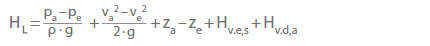
p    Static pressure
v    Flow velocity
z    Geodetic height
H_L  Head loss (see Pressure loss, Pressure head)
ρ    Density of fluid handled
g    Acceleration due to gravity

Location-specific subscripts

 e  Defined inlet cross-section (suction tank)
        See Head Fig. 2

a Defined outlet cross-section

s Pump suction nozzle

d Pump discharge nozzle

e,s Relate to the system's suction side, i.e. to the portion between the cross-sections e and s
        See Head Fig. 2

d,a  Relate to the system's discharge side, between the cross-sections d and a

The expression (v_a² – v_e²)/(2 ∙ g) is a negligible quantity if the system's cross-sections in e and a are of adequate size or of approximately the same size.

In practice, this expression is seldom of any significance. The expressions (p_a – p_e)/(ρ ∙ g) and (z_a – z_e) are independent of the pump's flow rate (Q).

Therefore, the relationship between the system head (H_sys) and the flow rate (Q) is evidenced mainly in the head losses (HL) which can be calculated by means of the following equation:

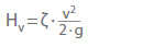
ζ   Loss coefficient (Head loss)
v   Flow velocity in a characteristic cross-section
    (of cross-sectional area A)

As the flow velocity (v) is the quotient of the flow rate (Q) and the cross-sectional area (A), and assuming a constant loss coefficient (ζ) and sufficiently high Reynolds numbers (see Model laws): we have: H_L ~ Q².

The reason for the system curve's parabola shape becomes clear. For the vertex of the system characteristic curve at Q = 0, we have:

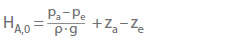
From the above equation it follows that the system characteristic curve shifts vertically in the H/Q_sys coordinate system if the system's tank pressures (p_a, p_e) and the geodetic head H_geo = z_a – z_e vary. H_sys,0 is often referred to as Hstat in the scholarly literature.

Thus for instance, we have the following equations for a cooling water system (see Cooling water pump), comprising a pipe drawing water out of a river, a cooling water pump and a discharge line leading into a cooling tower basin: See Fig. 1 System characteristic curve

H_A = z_a - z_e + H_v.e,s + H_v.d,a

H_A,0 = z_a - z_e

p_a = p_e = p_b    (see Atmospheric pressure)
v_a = 0             (negligible flow velocities at a)
v_e = 0             (negligible inlet velocities in the intake structure from
                      the river)
H_L Head loss  (pressure losses at inlet and outlet, pressure
                      losses through valves or elbows,
                       pressure losses caused by pipe friction, passage
                      through the condenser
                       and by abrupt changes of cross-section etc.)
z_a – z_e            Difference in geodetic head of the water level in the
                      cooling water basin and in the river bed.

As the water level in the river (z_e) fluctuates, the system characteristic curves will shift accordingly.
See Fig. 1 System characteristic curve