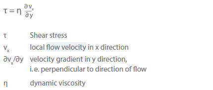
Viscosity is the property of a fluid, to resist the relative displacement of adjoining layers (internal friction). It is necessary to differentiate between dynamic andkinematic viscosity. The physical definition of viscosity originates in the NEWTONian formulation of shear stress (NEWTONian liquid).
The viscosity curve in the shear stress diagram (τ = f(∂vx/∂y)) is, therefore, a line through the origin, see Fig. 1 Pulp pumping. All other curves denote non-NEWTONian liquids handled in Pulp pumping applications, whose effects on the operation of centrifugal pumps cannot easily be calculated by the usual methods.
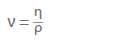
However, in practice it is normal to specify the viscosity-density ratio (kinematic viscosity).
The SI unit of dynamic viscosity is Ns/m2 = Pas, the SI unit of kinematic viscosity is m²/s.
The term "dynamic viscosity" is derived from the Greek "dynamis", which means force, since the SI unit contains a unit of force (N). The SI unit for kinematic viscosity, on the other hand, contains only kinematic dimensions for length (m) and time (s).
The dependence of kinematic viscosity ν on temperature t is shown both for water,
and for mineral oil distillates; with the axes being partitioned in such a way as to provide straight lines. See Fig. 1 Viscosity
Fig. 1 Viscosity: Kinematic viscosity v of various mineral oils as a function of temperature t
As the temperature increases, almost all liquids become thinner, i.e. their viscosity decreases. See Fig. 2 Viscosity
Fig. 2 Viscosity: Density ρ and kinematic viscosity v of various fluids as a function of temperature t
Dynamic viscosity η can be measured for all liquids using a rotational viscometer, in order to record the viscosity curve, as follows: a cylinder with freely selectable rotational speed rotates in a cylindrical pot filled with the liquid to be tested. Drive torque, circumferential speed, the size of the wetted cylinder surface and the wall clearance in the pot are measured at several rotational speeds. Viscometry also includes other processes, e.g. falling sphere and flow measuring methods.
Effect on the characteristic curves of pumps
Thecharacteristic curves of centrifugal pumps show noticeable effects only at a kinematic viscosity of
ν > 20 ·10 –6 m2/s and must be converted using empirically calculated conversion factors only after this limit is reached. The two most well-known techniques are those according to the Standards of the Hydraulic Institute (HI) and according to KSB. Both techniques use diagrams to illustrate the conversion factors, which - though they are used in a similar way - differ in that the KSB technique includes the influencing variables Q , H and ν as well as being clearly influenced by the specific rotational speed ns in addition. The HI technique, see Fig. 3 Viscosity, was measured only at ns = 15 to 20 rpm and, in this narrow application range, leads to similar results to the KSB technique see Fig. 4 Viscosity, which was measured in the ns range from 6.5 to 45 rpm and at viscosities of up to νz = 4000 · 10–6 m2/s. The use of the two diagrams is explained by means of the depicted examples.
Fig. 3 Viscosity: Diagram for the conversion of characteristic curves of centrifugal pumps with radial impellers pumping water to characteristic curves for pumping viscous fluids (from: Standards of the Hydraulic Institute, New York, USA 2004). Example shown for Q = 200 m³/h, H = 57 m, V =500 •10-6 m2/s
Fig. 4 Viscosity: Diagram for conversion of characteristic curves of centrifugal pumps with radial impellers for pumping higher-viscosity liquids (from: KSB). Example shown for Qw=200 m3/h, Hw=57,5 m, νz=500 • 10-6 m2/s, n=2900 min-1, ns,w=32,8 min-1, fη=0,61, fH=0,90, fQ=0,82
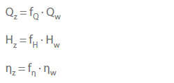
The capacity Q, the head H and the efficiency η of a single-stage centrifugal pump, which are known for operation with water (subscript W), can now be converted for operation with a viscous liquid (subscript Z) as follows:
The f factors are called k in the HI technique; both are illustrated graphically in Figures 3 and 4; in Fig. 4 Viscosity, in addition, the pump rotational speed n must be read in and the specific rotational speed ns of the pump impeller must be known.
With these factors, the operating data known for water mode can then be converted for liquids of a higher viscosity; the conversion applies in the load range:
0.8 Qopt < Q < 1.2 Qopt
Thus simplified at three flow rates 0.8 and 1.0 and 1.2 Qopt, with the only exception:
Q = 0.8 Qopt For Hz = 1.03 • fH • HW
At flow rate Q = 0, put simply:
Hz = Hw and ŋz =ŋw = 0
A calculation scheme simplifies the conversion. See Fig. 5 Viscosity
Fig. 5 Viscosity: Calculation template for converting pump characteristic curves for operation with higher-viscosity fluids, based on the KSB method
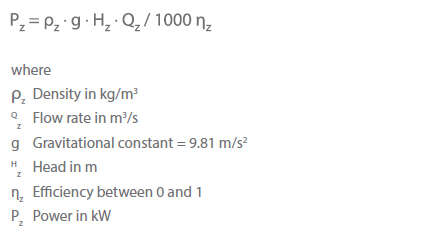
After the power at the three flow rates (see load range equation) has also been calculated according to
all characteristic curves can then each be plotted from either 4 or 3 calculated points over Qz. See Fig. 6 Viscosity
Fig. 6 Viscosity: Re-plotting the characteristic curves for water to those for a higher-viscosity liquid
If the terms of reference are reversed so that it is not the water values that are given, but the data for operation with a higher-viscosity liquid (e. g. to determine a suitable pump for a required duty point), the water values are first estimated and the solution is then approximated using the conversion factors fQ , fH and fη iteratively in two (or, if necessary, three) steps. Above a specific rotational speed of ns ≈ 20 rpm, the better adapted KSB calculation technique leads to lower drive ratings; below this limit the drive ratings calculated according to HI are too small!
Effect on the characteristic curves of the system
Since all hydrodynamic laws remain valid without restriction for NEWTONian liquids all the calculation formulae and diagrams for the pipe friction coefficients and for the loss coefficients in valves also continue to apply. It is only when calculating the REYNOLDS number Re = v · d/ν that, instead of the kinematic viscosity νw of water, νz, that of the respective higher-viscosity liquid must now be used, resulting in a lower Re number and consequently a greater pipe friction coefficient λz (see alsohead losses).
As an international employer, KSB offers exciting challenges in many different areas.
Regardless whether you are an experienced professional or a pupil, student or graduate ─ learn more about our work culture and find job openings from all over the world in our job portal.


. Example shown for Q = 200 m³/h, H = 57 m, V =500 •10<sup>-6</sup> m<sup>2</sup>/s")
. Example shown for Q<sub>w</sub>=200 m<sup>3</sup>/h, H<sub>w</sub>=57,5 m, ν<sub>z</sub>=500 • 10<sup>-6</sup> m<sup>2</sup>/s, n=2900 min<sup>-1</sup>, n<sub>s,w</sub>=32,8 min<sup>-1</sup>, f<sub>η</sub>=0,61, f<sub>H</sub>=0,90, f<sub>Q</sub>=0,82")